How Vector Databases Actually Find Your Nearest Neighbors

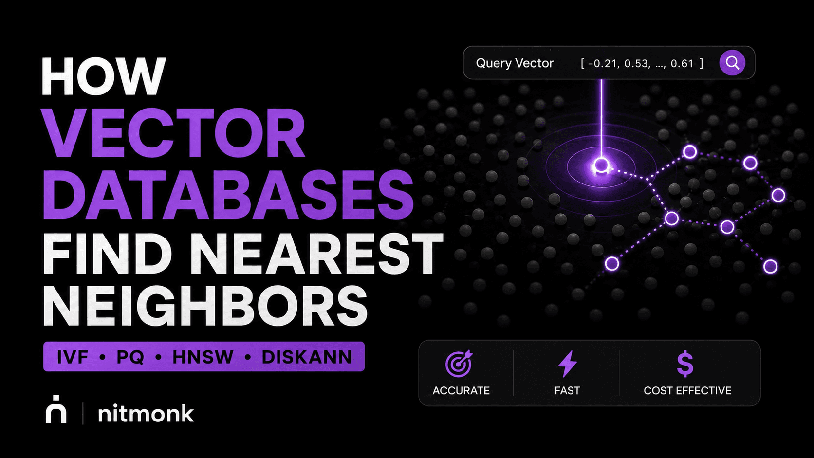
Ask a ten-million-document knowledge base a question, and an answer comes back in a few milliseconds. The first time you see it, it feels like magic. It isn't. It's an index that was built specifically to avoid comparing your query against most of the data.

Every AI engineer building RAG eventually hits the same wall: the naive version works on a thousand documents and falls over at ten million. Understanding why — and how real vector databases get around it — is the difference between a demo and a system that survives production. So let's walk through it, one search at a time.

First, what makes two vectors "similar"?

Before any clever indexing matters, two things have to be true: the numbers you're searching over must actually encode meaning, and "similar" has to mean something precise enough for a computer to calculate.

The first part is the embedding model's job. A sentence like "a red bicycle leaning on a wall" goes into a model and comes out as a point in a few hundred to a few thousand dimensions. The model is trained so that semantic closeness becomes geometric closeness — things that mean similar things land near each other. Every algorithm below depends on that holding true.

The second part is the distance function, and it's not one fixed idea:

• Cosine similarity measures the angle between two vectors, ignoring their length. It's the default for most modern text-embedding models, because magnitude usually encodes something other than meaning.
• Dot product is cosine's unnormalized cousin — cheaper to compute, and identical to cosine once vectors are normalized to unit length (which most databases do at insert time).
• Euclidean (L2) distance is straight-line distance. It shows up where magnitude itself is meaningful — some image embeddings and recommendation systems — rather than sentence embeddings.

Here's the trap: using a different distance function at query time than the model was trained with doesn't crash anything. It just quietly returns worse results. Match the metric to the model.

Brute force: correct, and too slow

The simplest possible search is a flat (brute-force) index: compare the query against every single vector, sort by distance, return the top k. It's exact — it always finds the true nearest neighbors — which makes it the ground truth every other method is measured against.

It's also linear. Ten thousand vectors? Fine. Ten million vectors at 768 dimensions? You're doing billions of floating-point operations per query, and latency climbs with your data. Flat search is perfect for small collections and for evaluating recall. It does not scale.

So every production index makes the same bet: give up a tiny bit of accuracy to skip almost all of the work. This is called Approximate Nearest Neighbor (ANN) search, and here are the four ideas that power it.

IVF: skip the clusters that can't hold your answer

Inverted File (IVF) indexes cluster your vectors ahead of time — say, into a few thousand groups, each with a representative centroid. At query time, you compare the query only to the centroids, pick the handful of nearest clusters, and search only inside those.

The knob is nprobe: how many clusters to actually look in. Probe more clusters and recall goes up but so does latency; probe fewer and it's faster but you risk missing neighbors that sit just across a cluster boundary. IVF is simple, memory-friendly, and a great default at moderate scale.

Product quantization: shrink every vector

The problem at scale often isn't just compute — it's memory. A billion 768-dimensional float32 vectors is multiple terabytes of RAM. Product Quantization (PQ) attacks that directly: it chops each vector into sub-vectors, and replaces each sub-vector with the id of the nearest entry in a small learned codebook.

The result is dramatic compression — a vector that took kilobytes now fits in a few dozen bytes — so far more data fits in memory, and distance calculations run on the compact codes. You trade some precision for a massive footprint reduction, which is why PQ is usually combined with IVF (IVF-PQ) rather than used alone.

HNSW: navigate a graph of shortcuts

Hierarchical Navigable Small World (HNSW) is the algorithm most people mean when they say "fast vector search." Instead of clustering, it builds a multi-layer graph: the top layers are sparse with long-range links, the bottom layer is dense with every node.

A search starts at the top, greedily hops toward the query along the long links to get into the right neighborhood fast, then drops a layer and refines — like zooming from country to city to street. It reaches excellent recall in a logarithmic number of hops instead of a linear scan.

The catch is memory and build cost: HNSW keeps the whole graph in RAM and is more expensive to construct and update. For most in-memory workloads, it's the accuracy-latency sweet spot — which is why nearly every database below offers it.

DiskANN: when the index won't fit in memory

What happens when even a compressed index is too big for RAM? DiskANN builds a graph index that lives on SSD, keeping only a compressed version of the vectors in memory to guide the walk and reading the full vectors from disk only for the few candidates it actually needs to score.

It's how you serve billion-scale collections on a single machine without a RAM budget that dwarfs your compute bill. The tradeoff is added latency from disk reads, carefully engineered to stay in the low-milliseconds range.

Filtering changes everything

Here's the part tutorials skip: similarity search is almost never just similarity. In the real world you want "the nearest neighbors from this user's documents, published this year, in English." The moment you add a metadata filter, the naive approaches break in subtle ways:

• Post-filtering (retrieve by similarity, then throw away non-matches) can return too few results — or none — if your filter is selective.
• Pre-filtering (find matches first, then search) can be slow if the matching set is huge.

The best systems push the filter into the search itself — for example, filtering during the HNSW graph walk so it never wastes hops on vectors that can't qualify. When you evaluate a vector database, its filtered search quality matters as much as its raw ANN speed.

The tradeoff you can never escape

Strip away the names and every one of these algorithms is negotiating the same triangle:

• Recall — did you actually find the true nearest neighbors?
• Latency — how fast did the query return?
• Memory/cost — how much RAM and disk did it take?

You cannot maximize all three. IVF and HNSW trade recall for speed via their knobs; PQ trades precision for memory; DiskANN trades latency for cost. Picking a vector database is really about which corner of that triangle your product can least afford to give up.

Six vector databases, compared

A vector database wraps one or more of these indexes with storage, filtering, and operations. The right choice usually has less to do with raw speed and more to do with what you're already running and how much infrastructure you want to own.

• pgvector — a Postgres extension. Best if you're already on PostgreSQL at moderate scale. Indexes: Flat, IVFFlat, HNSW. Filtering is native SQL WHERE; hybrid search means pairing with Postgres full-text search. Lowest operational load — one less system to run. Practical scale: tens of millions on a single node.
• Pinecone — fully managed and serverless. Best for production RAG when you want zero infra to run. The ANN is proprietary and not user-selectable; filtering and sparse-dense hybrid are native. Scales automatically into the billions. You trade control and per-unit cost for near-zero operations.
• Qdrant — a performance-focused OSS engine written in Rust. Best for performance-sensitive self-hosting. HNSW plus scalar/binary/product quantization, with filtering built into the HNSW walk itself. Moderate operational load — you run and tune it. Hundreds of millions per cluster.
• Weaviate — OSS with hybrid search as a first-class feature. Best for apps that need semantic and keyword (BM25 + vector) fusion, with per-property inverted indexes for filtering and built-in multi-tenancy. Self-hosted or managed.
• Milvus — distributed OSS built for massive scale. The richest index menu (HNSW, IVF, IVF-PQ, DiskANN, and more) with compute and storage that scale independently. Highest operational load — it's a distributed system to operate — but it reaches billions to tens of billions. There's a Milvus Lite for laptops.
• Elasticsearch / OpenSearch — a full search engine with vector search bolted on via a k-NN plugin. Best when you already need BM25, aggregations, or logs and want vectors in the same place. Mature filtered search and first-class hybrid retrieval, proven at large search scale.

One honest caveat: these are design-center characterizations, not benchmark results. A well-tuned pgvector deployment can beat a poorly-tuned distributed cluster, and vice versa. Cost, latency, and recall depend heavily on your data, dimensionality, filter selectivity, and configuration. Before you bet production on any single number, run your own benchmark on your own data and filters.

When to reach for each one

The question is rarely "which is fastest?" It's "which fits my constraints?"

• Already on Postgres, moderate scale? Start with pgvector. Not adding a new system is worth a lot.
• Want production RAG with no infra to babysit? Pinecone.
• Self-hosting and latency-sensitive? Qdrant.
• Need real hybrid (keyword + semantic) search? Weaviate.
• Genuinely huge, distributed, GPU-scale? Milvus.
• Already running Elastic/OpenSearch for logs or BM25? Use its k-NN and keep everything in one place.

Where this fits in your RAG pipeline

Retrieval quality is the single biggest lever on whether a RAG system hallucinates. The vector index is what decides which chunks your model even sees — and now you know it's not magic, it's an engineering decision about recall, latency, and cost.

If you want to watch these ideas run visually — brute force vs. HNSW on the same query — I broke it down in my video, How Vector Databases Actually Work. And when you're ready to test yourself on this and the rest of the RAG stack, the LLM & RAG Fundamentals quiz covers embeddings, chunking, and vector search end to end.

Build the intuition once, and every vector database stops looking like a black box.